%matplotlib inline

Train Node Classification Model without Graph

Node classification model can be realised with neural networks with Fully-Connected Layers (FCNs) without using graph models. However, in our manuscript, we demonstrated that the graph model based on Neighborhood Gene Component has the advantage of message passing, so that the predicted labels of neighboring transcripts are similar. Here we use 10x Xenium DCIS data [Janesick et al., 2022] as an example to demonstrate the advantage of graph models in the node (transcript) classification.

Import packages & data

import random
import numpy as np
import pandas as pd
import matplotlib.pyplot as plt 

import Bering as br

load data

df_spots_all = br.datasets.xenium_dcis_janesick()
df_spots_seg = df_spots_all[df_spots_all['labels'] != 'background'] # foreground nodes
df_spots_unseg = df_spots_all[df_spots_all['labels'] == 'background'] # background nodes

Create Bering object and training data

# image-dependent segmentation
bg = br.BrGraph(df_spots_seg, df_spots_unseg)
br.graphs.BuildWindowGraphs(bg, n_cells_perClass = 10, window_width = 15.0, window_height = 15.0, n_neighbors = 30)
br.graphs.CreateData(bg, batch_size = 16, training_ratio = 0.8)

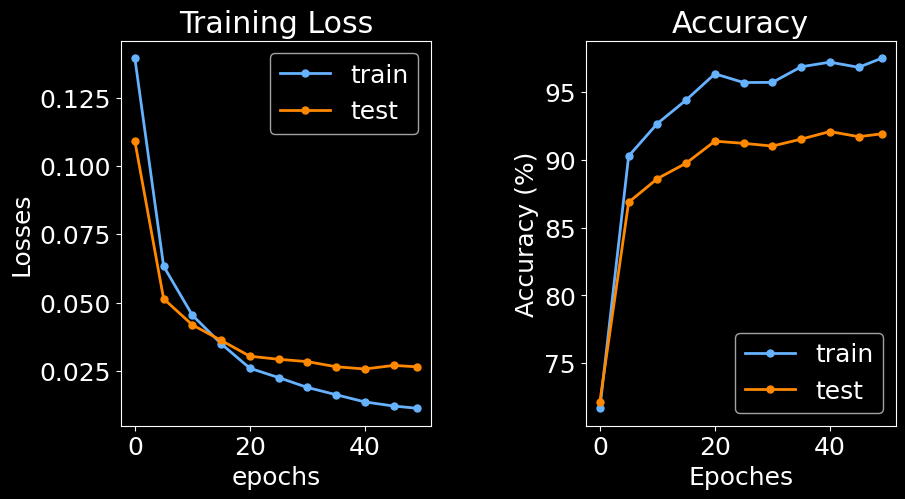
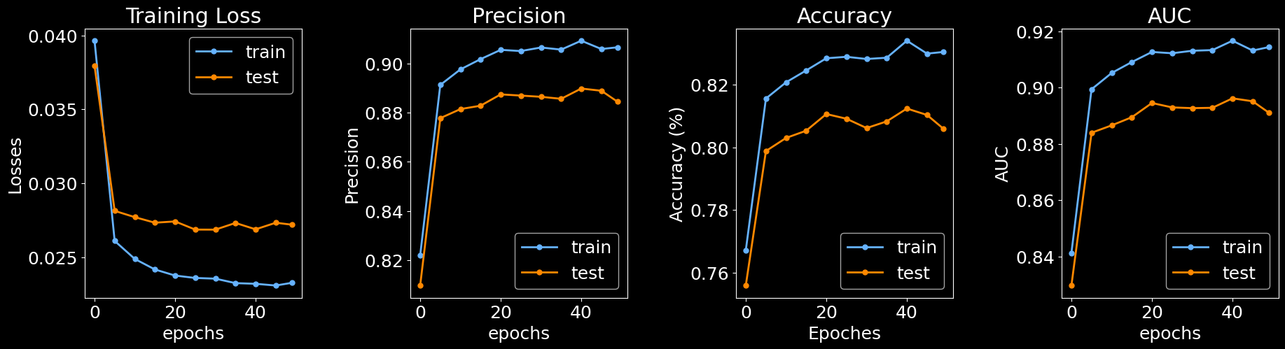
Training (without Graph)

br.train.Training(bg, baseline = True)

Training node classifier:  98%|█████████▊| 49/50 [00:38<00:00,  1.65it/s]

Training node classifier: 100%|██████████| 50/50 [00:40<00:00,  1.22it/s]
Training edge classifier:  98%|█████████▊| 49/50 [01:08<00:01,  1.22s/it]

Training edge classifier: 100%|██████████| 50/50 [01:11<00:00,  1.42s/it]

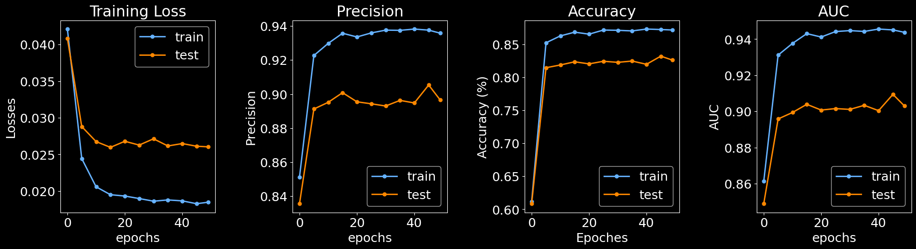
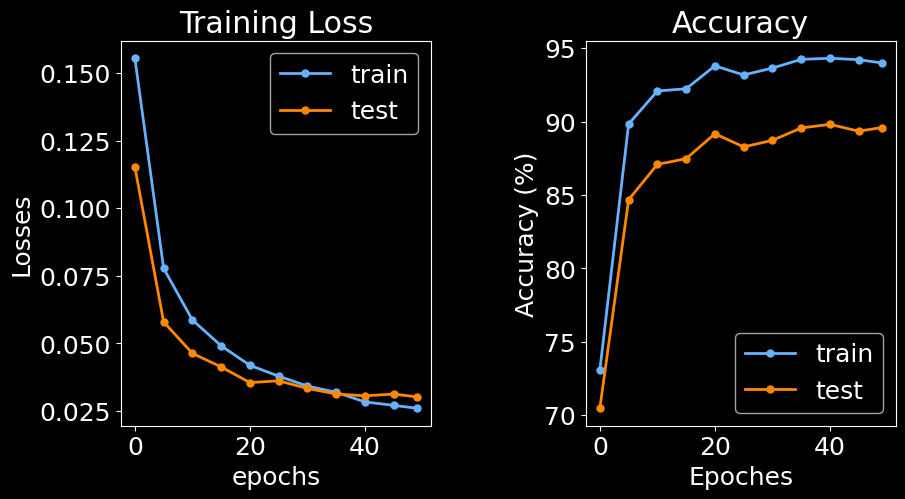
Training (with graph)

# image-dependent segmentation
bg_graph = br.BrGraph(df_spots_seg, df_spots_unseg)
br.graphs.BuildWindowGraphs(bg_graph, n_cells_perClass = 10, window_width = 15.0, window_height = 15.0, n_neighbors = 30)
br.graphs.CreateData(bg_graph, batch_size = 16, training_ratio = 0.8)
br.train.Training(bg_graph, baseline = False)

Training node classifier:  98%|█████████▊| 49/50 [01:28<00:01,  1.44s/it]

Training node classifier: 100%|██████████| 50/50 [01:35<00:00,  1.90s/it]
Training edge classifier:  98%|█████████▊| 49/50 [01:36<00:01,  1.74s/it]

Training edge classifier: 100%|██████████| 50/50 [01:40<00:00,  2.01s/it]

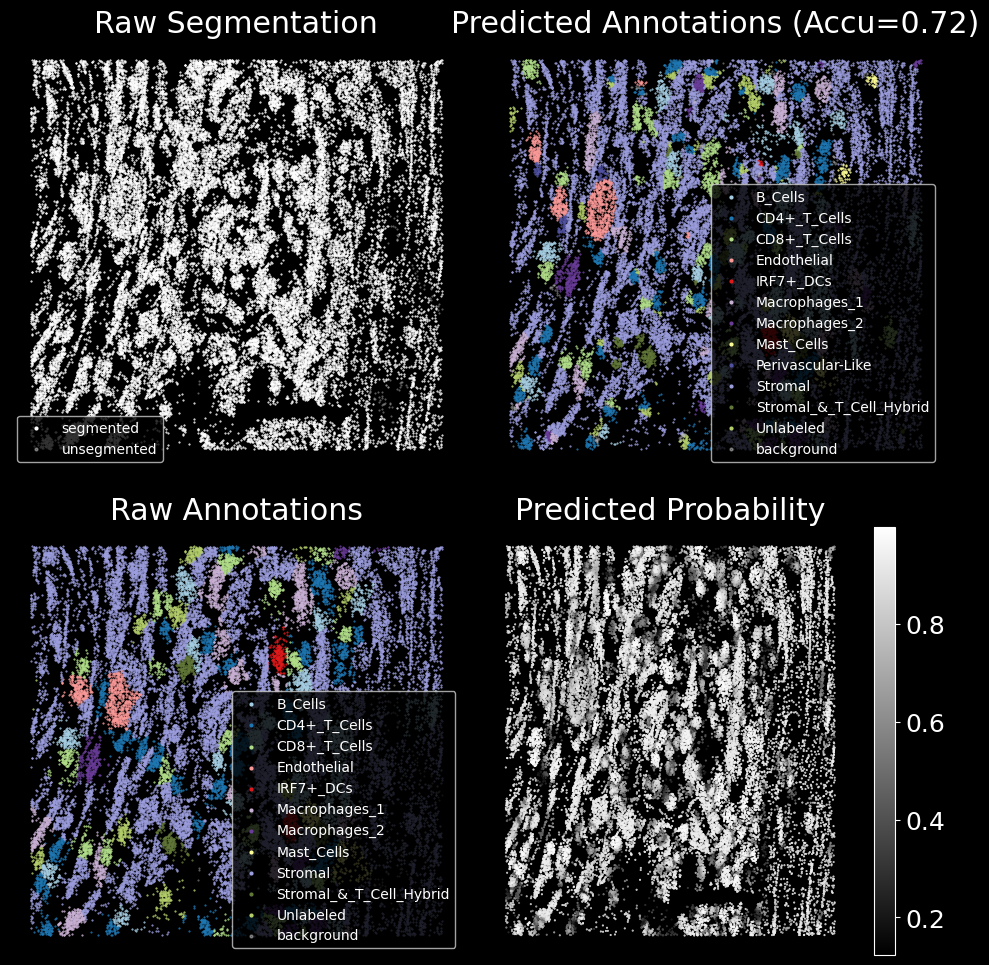
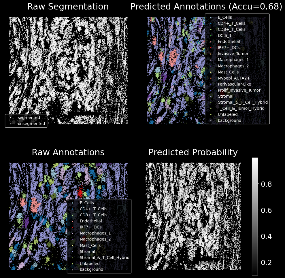
Comparison of two predictions

# randomly select a cell
random.seed(42)
random_cell = cells = random.sample(bg.segmented.index.values.tolist(), 1)[0]

# plot node classification
_,_,_ = br.pl.Plot_Classification(
    bg, 
    cell_name = random_cell,
    n_neighbors = 30, 
    zoomout_scale = 8,
)

# plot node classification
_,_,_ = br.pl.Plot_Classification(
    bg_graph, 
    cell_name = random_cell,
    n_neighbors = 30, 
    zoomout_scale = 8,
)