%matplotlib inline
Visualize Single Cell Data Using Segmentation Results
This tutorial shows how to utilize segmentation results to conduct downstream single cell analysis. The single-cell analysis part requires popularly used packages scanpy and anndata.
Here we use 10x Xenium DCIS data as an example. We mainly focus on how the segmentation results can be used for downstream single-cell analysis. The steps of model training are skipped and more details can be accessed from xxx.
Import packages & data
import sys
import random
import numpy as np
import pandas as pd
import tifffile as tiff
import matplotlib.pyplot as plt

sys.path.append('/data/aronow/Kang/spatial/Bering/cosmx')
import BeringNodeToLink_v3 as br
After the model is trained, we can use the trained model to predict the cell types and segment all spots on the whole slice. After node classification and cell segmentation is completed, we generate single cell matrix in the end.
load pretrained model
import pickle
with open('/data/aronow/Kang/spatial/Bering/demo/tutorials/plotting/models/Xenium_dcis_model_simplified.pl', 'rb') as f:
    bg = pickle.load(f)
Get single cell data from whole slice
In the function br.tl.cell_annotation, we generate two single cell data, including one from direct prediction result, and the other from ensembl annotations of the prediction. More details can be found in the function description.
br.tl.node_classification(bg, bg.spots_all.copy(), n_neighbors = 30)
br.tl.cell_segmentation(bg)
df_results, adata_ensembl, adata_segmented = br.tl.cell_annotation(bg)

print(adata_segmented.shape)
print(adata_segmented.obs.head())
print(adata_ensembl.shape)
print(adata_ensembl.obs.head())
                     x          y          z features  segmented   labels  \
molecule_id
0            2100.0261  2350.3684  19.269732      LUM          0  Stromal
1            2100.2126  2178.9346  18.475246   HAVCR2          1  Stromal
2            2100.3599  2261.9116  20.490784    RUNX1          2  Stromal
3            2100.3918  2155.2341  20.006990     TCIM          3  Stromal
4            2100.5117  2353.7695  20.749512    CXCR4          4  B_Cells

                groups predicted_node_labels  predicted_probability  \
molecule_id
0            segmented               Stromal               0.863927
1            segmented         Macrophages_2               0.326667
2            segmented               Stromal               0.899313
3            segmented               Stromal               0.667508
4            segmented               Stromal               0.667900

             predicted_cells_resolution=0.01  predicted_cells  \
molecule_id
0                                        489              489
1                                        320              320
2                                        370              370
3                                        313              313
4                                        489              489

             ensembled_cells ensembled_labels
molecule_id
0                        489          Stromal
1                        320          Stromal
2                        370          Stromal
3                        313          Stromal
4                        489          Stromal
(7535, 540)
    n_counts  n_genes           cx           cy
-1      4757      297  2455.268227  2433.417828
0       3396      194  2374.655610  2280.935440
1       3380      227  2371.465405  2121.776126
2       3358      250  2841.205267  2688.078428
3       3327      265  2868.166271  2333.154009
(857, 540)
   n_counts  n_genes           cx           cy predicted_labels
0      3396      194  2374.655610  2280.935440   Invasive_Tumor
1      3380      227  2371.465405  2121.776126   Invasive_Tumor
2      3358      250  2841.205267  2688.078428          Stromal
3      3327      265  2868.166271  2333.154009          Stromal
4      3219      203  2815.938887  2520.709648          Stromal
Single cell data analysis
# define function for single cell analysis from raw count matrix
import scanpy as sc
def sc_analysis(adata):
sc.pp.filter_cells(adata, min_counts = 10)
sc.pp.normalize_total(adata, target_sum = 1e3)
sc.pp.log1p(adata)
sc.pp.scale(adata) # the number of features is less than 1000, so we don't use variable genes here
sc.tl.pca(adata)
sc.pp.neighbors(adata, n_neighbors = 10)
sc.tl.umap(adata)
sc.tl.leiden(adata)
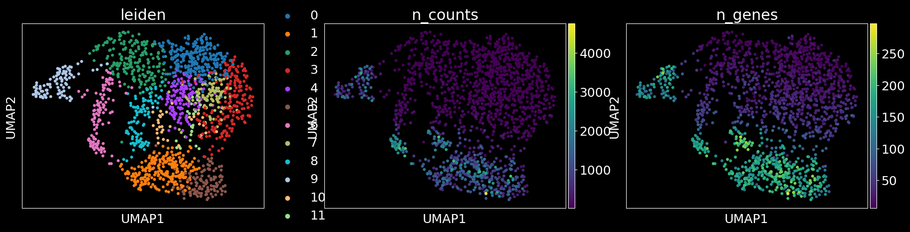
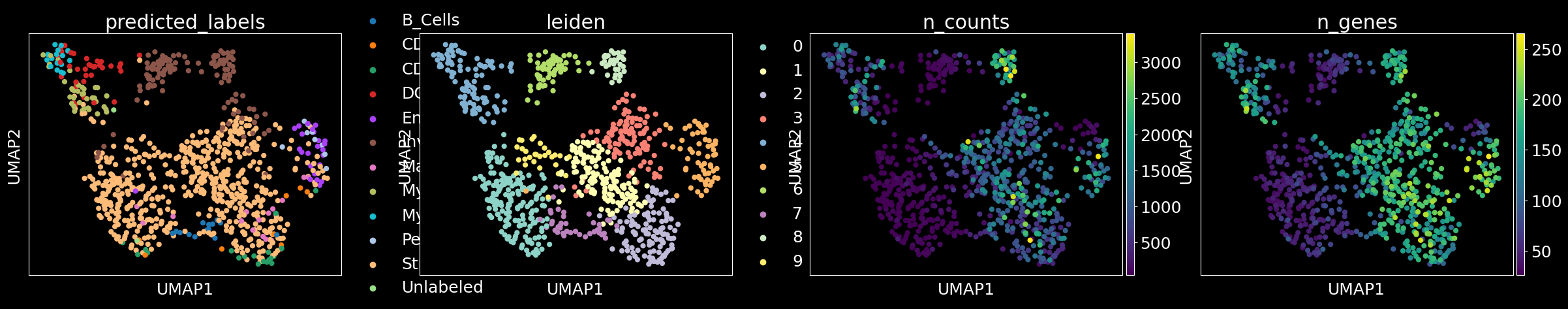
# plot Bering results and Leiden clustering
columns = ['predicted_labels','leiden','n_counts','n_genes'] if 'predicted_labels' in adata.obs.columns else ['leiden','n_counts','n_genes']
sc.pl.umap(adata, color = columns)
# analysis of segmented cells without ensembl annotations
sc_analysis(adata_segmented)
2023-07-03 17:20:19.840255: I tensorflow/core/platform/cpu_feature_guard.cc:193] This TensorFlow binary is optimized with oneAPI Deep Neural Network Library (oneDNN) to use the following CPU instructions in performance-critical operations:  AVX2 AVX512F AVX512_VNNI FMA
To enable them in other operations, rebuild TensorFlow with the appropriate compiler flags.
2023-07-03 17:20:20.690205: I tensorflow/core/util/port.cc:104] oneDNN custom operations are on. You may see slightly different numerical results due to floating-point round-off errors from different computation orders. To turn them off, set the environment variable `TF_ENABLE_ONEDNN_OPTS=0`.
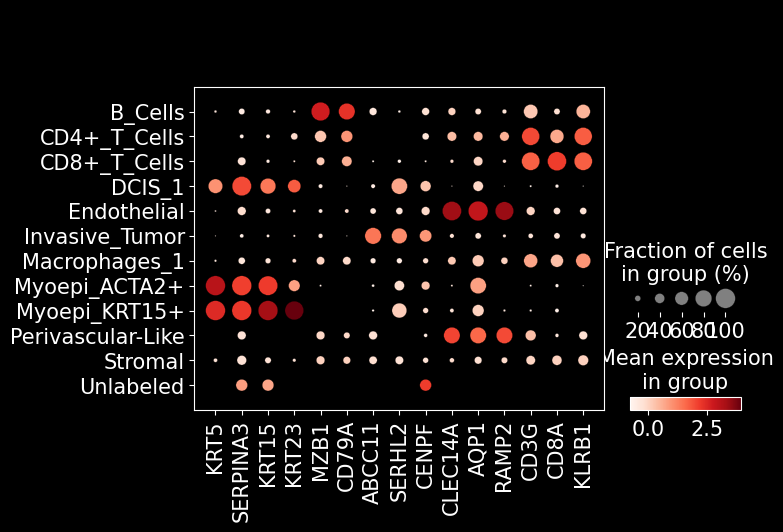
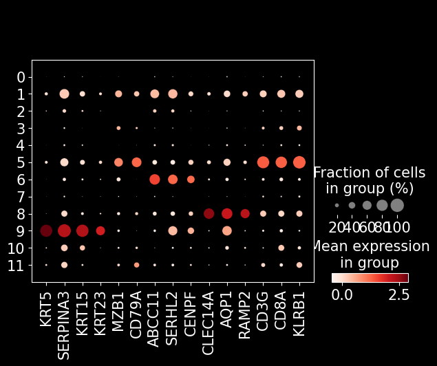
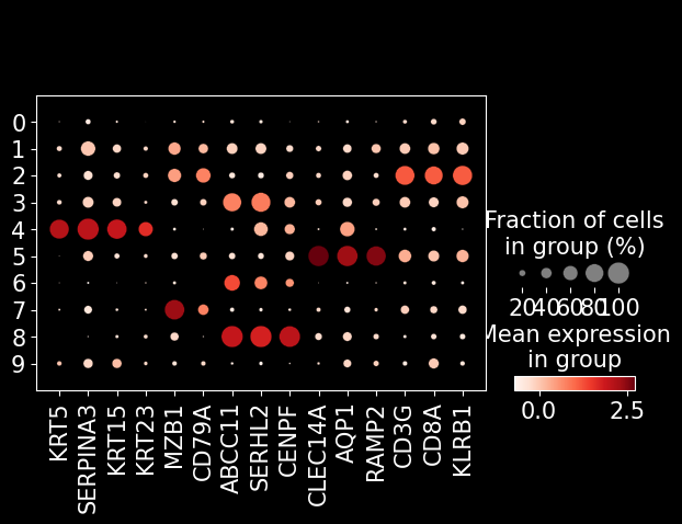
marker_genes = [
    'KRT5', 'SERPINA3', 'KRT15', 'KRT23', # tumor
    'MZB1', 'CD79A', # pDC
    'ABCC11', 'SERHL2', 'CENPF', # epithelial
    'CLEC14A', 'AQP1', 'RAMP2', # endothelial
    'CD3G', 'CD8A', 'KLRB1', # T cell
]
sc.pl.dotplot(adata_segmented, marker_genes, groupby = 'leiden')
# analysis of segmented cells with ensembl annotations
sc_analysis(adata_ensembl)
... storing 'predicted_labels' as categorical
sc.pl.dotplot(adata_ensembl, marker_genes, groupby = 'leiden')
sc.pl.dotplot(adata_ensembl, marker_genes, groupby = 'predicted_labels')