%matplotlib inline

Analyze MERFISH Mouse Cortex data

This tutorial shows how to apply Bering to MERFISH data.

MERFISH mouse cortex data [Zhang et al., 2021], which contains transcripts which were segmented vs. unsegmented in the original paper. Coordinates (x, y, z (optional)) and gene names are required for all nodes. For segmented transcripts, we additionally require information about segmented cell id and labels.

Import packages & data

import random
import pandas as pd
import matplotlib as mpl
import matplotlib.pyplot as plt 

import Bering as br

mpl.rcParams['figure.figsize'] = [3.5, 3.5]

# load data
df_spots_all = br.datasets.merfish_cortex_zhang()
df_spots_seg = df_spots_all[df_spots_all['labels'] != 'background'] # foreground nodes
df_spots_unseg = df_spots_all[df_spots_all['labels'] == 'background'] # background nodes
df_spots_seg.head()

Downloading dataset `merfish_cortex_zhang` from `https://figshare.com/ndownloader/files/41409090` as `None.tsv`

	x	y	z	features	segmented	labels
5163158	-4146.0044	1027.1519	0.0	Aqp4	187427829321727974677294895804085147126	VLMC
5163175	-4147.0884	1028.8763	0.0	Igf2	187427829321727974677294895804085147126	VLMC
5163190	-4145.6426	1028.3645	0.0	Nr2f2	187427829321727974677294895804085147126	VLMC
5163198	-4143.3530	1025.8699	0.0	Rgs6	187427829321727974677294895804085147126	VLMC
5163200	-4145.2314	1026.4473	0.0	Serpinf1	187427829321727974677294895804085147126	VLMC

df_spots_unseg.head() # visualize unsegmented data

	x	y	z	features	segmented	labels
5163155	-4116.2620	918.22800	0.0	Aqp4	-1	background
5163156	-4145.6465	931.03687	0.0	Aqp4	-1	background
5163157	-4192.2363	1023.08344	0.0	Aqp4	-1	background
5163159	-4193.5073	1029.53480	0.0	Aqp4	-1	background
5163160	-4092.1545	1017.06165	0.0	Bgn	-1	background

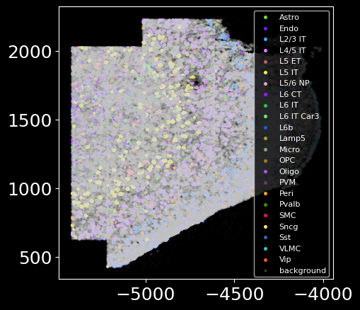
# visualize segmented and unsegmented data
br.pl.Plot_Spots(df_spots_seg = df_spots_seg, df_spots_unseg = df_spots_unseg)

Create Bering object

img = None; channels = None # image-free segmentation in this case
bg = br.BrGraph(
    df_spots_seg, df_spots_unseg, img, channels,
)
bg

<Bering.objects.bering.Bering_Graph at 0x2b8d5b277c70>

bg.segmented.head() # summary of cells

	cx	cy	cz	dx	dy	dz	d	labels
segmented
0	-4147.2183	1029.63480	3.0	9.2470	6.2306	6.0	9.2470	VLMC
1	-4140.8835	1121.99090	4.5	16.9153	7.4033	7.5	16.9153	SMC
2	-4139.7197	1130.35130	6.0	29.8024	23.6521	7.5	29.8024	VLMC
3	-4158.9525	1081.01685	4.5	19.1810	12.3783	7.5	19.1810	VLMC
4	-4153.4095	1092.16530	4.5	11.9056	11.9655	7.5	11.9655	VLMC

Create training data

# Build graphs for GCN training purpose
br.graphs.BuildWindowGraphs(
    bg, 
    n_cells_perClass = 30, 
    window_width = 50.0, 
    window_height = 50.0, 
    n_neighbors = 30, 
    use_unsegmented_ratio = 0.5, # use 50% of unsegmented spots to avoid learning too much knwoledge from unsegmented spots / noises
)

br.graphs.CreateData(
    bg, 
    batch_size = 16, 
    training_ratio = 0.8, 
)

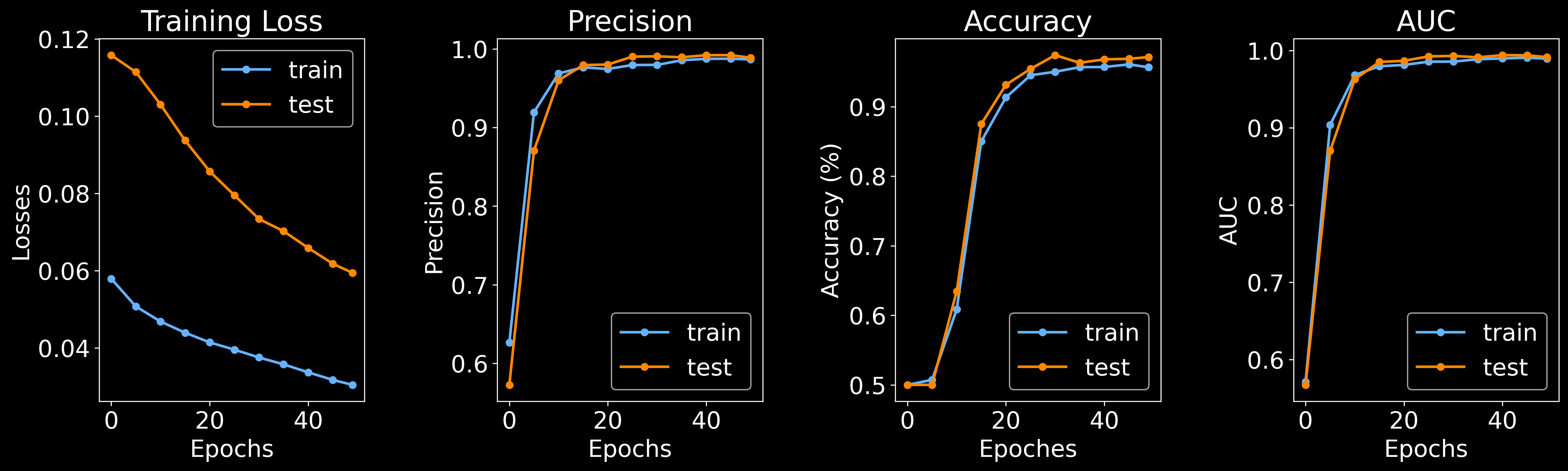
Training

br.train.Training(
    bg,
    node_gcnq_hidden_dims = [512, 256, 128, 128, 64, 64, 32, 16],
    node_foreground_weight = 2.0,
    node_background_weight = 1.0,
    edge_rbf_start = 0,
    edge_rbf_stop = 64,
    edge_rbf_n_kernels = 32,
    node_epoches = 100,
)

Training node classifier:  99%|█████████████████████████████████████████████████████████████████████████████████████████████████ | 99/100 [00:39<00:00,  2.71it/s]

Training node classifier: 100%|█████████████████████████████████████████████████████████████████████████████████████████████████| 100/100 [00:41<00:00,  2.42it/s]
Training edge classifier:  98%|█████████████████████████████████████████████████████████████████████████████████████████████████  | 49/50 [00:22<00:00,  3.65it/s]

Training edge classifier: 100%|███████████████████████████████████████████████████████████████████████████████████████████████████| 50/50 [00:24<00:00,  2.07it/s]

# save the trained model
import pickle
with open('merfish_cortex_zhang.pkl', 'wb') as f:
    pickle.dump(bg, f)

Visualizing model

# randomly select a cell
random_cell = cells = random.sample(bg.segmented.index.values.tolist(), 1)[0]

# plot node classification
_ = br.pl.Plot_Classification(
    bg, 
    cell_name = random_cell,
    n_neighbors = 30, 
    zoomout_scale = 12,
)

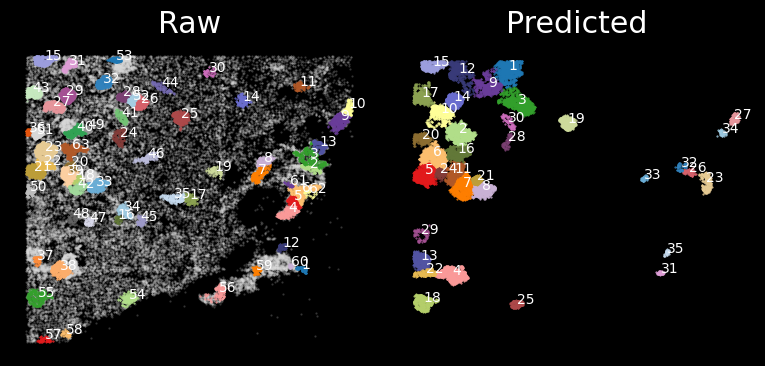
# plot cell segmentation (original and predicted cells are on left and right, respectively)
random_cells = cells = random.sample(bg.segmented.index.values.tolist(), 1)[:3]
for random_cell in random_cells:
    print(f'Plotting segmentation for the region around cell {random_cell}')
    br.pl.Plot_Segmentation(
        bg, 
        cell_name = random_cell,
        n_neighbors = 30, 
        zoomout_scale = 12,
        use_image = False,
        pos_thresh = 0.7,
        resolution = 0.02,
        num_edges_perSpot = 100,
        min_prob_nodeclf = 0.3,
        n_iters = 20,
    )

Plotting segmentation for the region around cell 285

After the model is trained, we can use the trained model to predict the cell types and segment all spots on the whole slice. After node classification and cell segmentation is completed, we generate single cell matrix in the end.

Node classification

Conduct node classification on the whole slice.

br.tl.node_classification(
    bg, bg.spots_all.copy(), 
    n_neighbors = 30, 
)
bg.spots_all.to_csv('spots_all.txt', sep = '\t')

Cell segmentation

br.tl.cell_segmentation(bg)

Get single cells

df_results, adata_ensembl, adata_segmented = br.tl.cell_annotation(bg)
df_results.to_csv('results.txt', sep = '\t')
adata_ensembl.write('results_cells_ensembled.h5ad')
adata_segmented.write('results_cells_segmented.h5ad')

print(f'Ensembled anndata: {adata_ensembl.shape}')
print(f'Segmented anndata: {adata_segmented.shape}')

... storing 'predicted_labels' as categorical

Ensembled anndata: (724, 252)
Segmented anndata: (1028, 252)

Single cell data analysis

import scanpy as sc
sc.settings.set_figure_params(dpi=80)

# run standard analysis on the ensembled anndata
adata_ensembl = br.tl.cell_analyze(adata_ensembl)

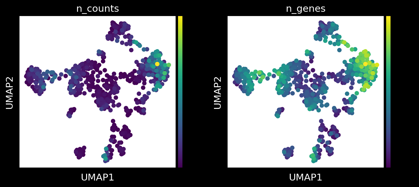
# first check the data quality of segmented cells
sc.pl.umap(adata_ensembl, color = ['n_counts','n_genes'])

2023-08-22 14:55:30.159333: I tensorflow/core/platform/cpu_feature_guard.cc:193] This TensorFlow binary is optimized with oneAPI Deep Neural Network Library (oneDNN) to use the following CPU instructions in performance-critical operations:  AVX2 AVX512F AVX512_VNNI FMA
To enable them in other operations, rebuild TensorFlow with the appropriate compiler flags.
2023-08-22 14:55:30.395720: I tensorflow/core/util/port.cc:104] oneDNN custom operations are on. You may see slightly different numerical results due to floating-point round-off errors from different computation orders. To turn them off, set the environment variable `TF_ENABLE_ONEDNN_OPTS=0`.

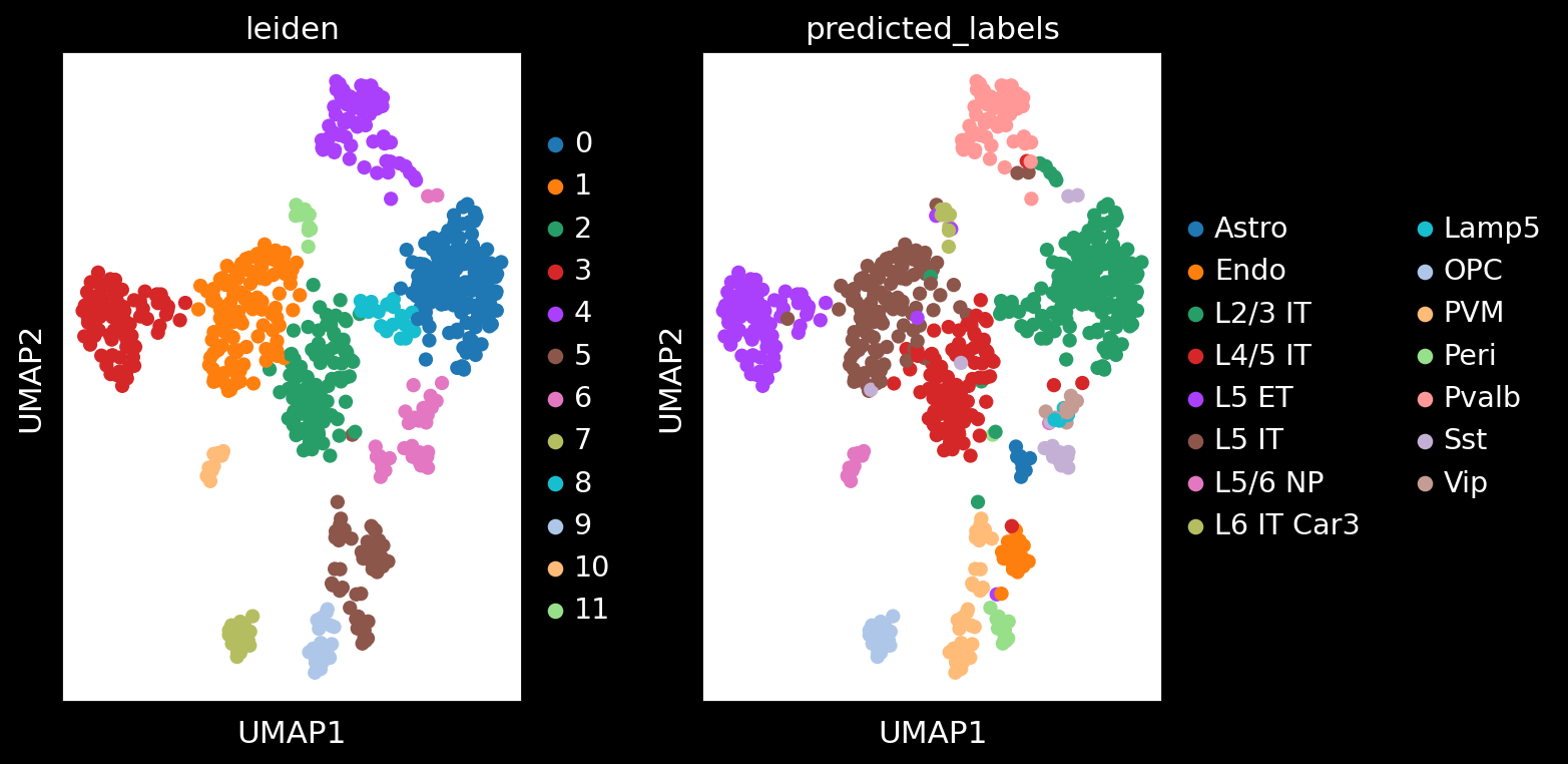
# plot leiden clustering and predicted labels from Bering
fig, axes = plt.subplots(1, 2, figsize = (10, 5))
axes[0] = sc.pl.umap(adata_ensembl, color = ['leiden'], ax = axes[0], show = False)
axes[1] = sc.pl.umap(adata_ensembl, color = ['predicted_labels'], ax = axes[1], show = False)

plt.subplots_adjust(wspace = 0.5)
plt.tight_layout()
plt.show()