%matplotlib inline

Analyze MERFISH ileum data

This tutorial shows how to apply Bering to MERFISH ileum data.

MERFISH ileum [Petukhov et al., 2022] data was derived from: https://datadryad.org/stash/dataset/doi:10.5061/dryad.jm63xsjb2. The data include spatial distribution of transcripts from 241 genes, and DAPI and membrane staining images.

Import packages & data

import random
import pandas as pd
import matplotlib as mpl
import matplotlib.pyplot as plt 

import Bering as br

mpl.rcParams['figure.figsize'] = [3.5, 3.5]

# load data
df_spots_all = br.datasets.merfish_ileum_petukhov()
df_spots_seg = df_spots_all[df_spots_all['labels'] != 'background'] # foreground nodes
df_spots_unseg = df_spots_all[df_spots_all['labels'] == 'background'] # background nodes
img = None # image-free
channels = None

df_spots_seg.head()

Downloading dataset `merfish_ileum_petukhov` from `https://figshare.com/ndownloader/files/41409102` as `None.tsv`

	x	y	z	features	segmented	labels
mol_id
3048145	1705.0	1271.0	0.0	Maoa	84	Smooth Muscle
3048147	1725.0	1922.0	0.0	Maoa	231	Myenteric Plexus
3048148	1753.0	1863.0	0.0	Maoa	231	Myenteric Plexus
3048149	1760.0	1865.0	0.0	Maoa	231	Myenteric Plexus
3048153	1904.0	794.0	0.0	Maoa	53	Smooth Muscle

df_spots_unseg.head() # visualize unsegmented data

	x	y	z	features	segmented	labels
mol_id
3048188	1781.0	1101.0	55.072763	Maoa	-1	background
3048192	1896.0	660.0	55.072763	Maoa	-1	background
3048255	1682.0	1382.0	13.768191	Txndc5	-1	background
3048374	1893.0	1563.0	0.000000	Slc12a2	-1	background
3048376	1910.0	1472.0	0.000000	Slc12a2	-1	background

br.pl.Plot_Spots(df_spots_seg = df_spots_seg, df_spots_unseg = df_spots_unseg)

Create Bering object

# image-dependent segmentation
bg = br.BrGraph(df_spots_seg, df_spots_unseg, img, channels)
bg

<Bering.objects.bering.Bering_Graph at 0x2b17f4d52310>

bg.segmented.head() # summary of cells

	cx	cy	cz	dx	dy	dz	d	labels
segmented
0	1710.0	1263.0	55.072763	77.0	76.0	96.377334	96.377334	Smooth Muscle
1	1742.0	1895.0	27.536381	105.0	121.0	82.609144	121.000000	Myenteric Plexus
2	1928.0	837.0	27.536381	156.0	120.0	96.377334	156.000000	Smooth Muscle
3	1899.5	1414.0	27.536381	139.0	89.0	82.609144	139.000000	Smooth Muscle
4	1812.5	1849.0	27.536381	74.0	54.0	55.072763	74.000000	Myenteric Plexus

Create training data

# Build graphs for GCN training purpose
br.graphs.BuildWindowGraphs(
    bg, 
    n_cells_perClass = 5, 
    window_width = 150.0, 
    window_height = 150.0, 
    n_neighbors = 10, 
)

br.graphs.CreateData(
    bg, 
    batch_size = 16, 
    training_ratio = 0.8, 
)

Training

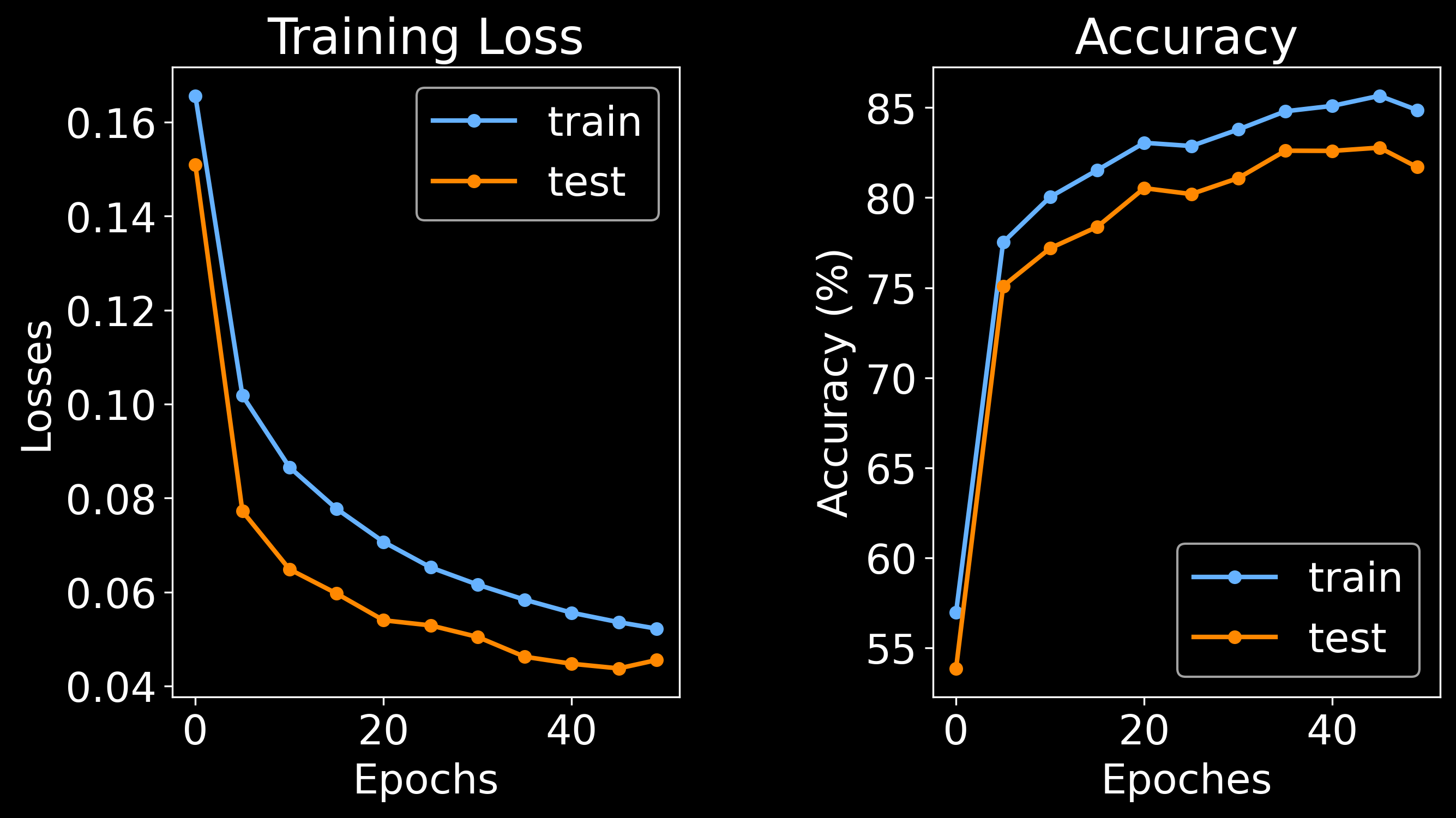
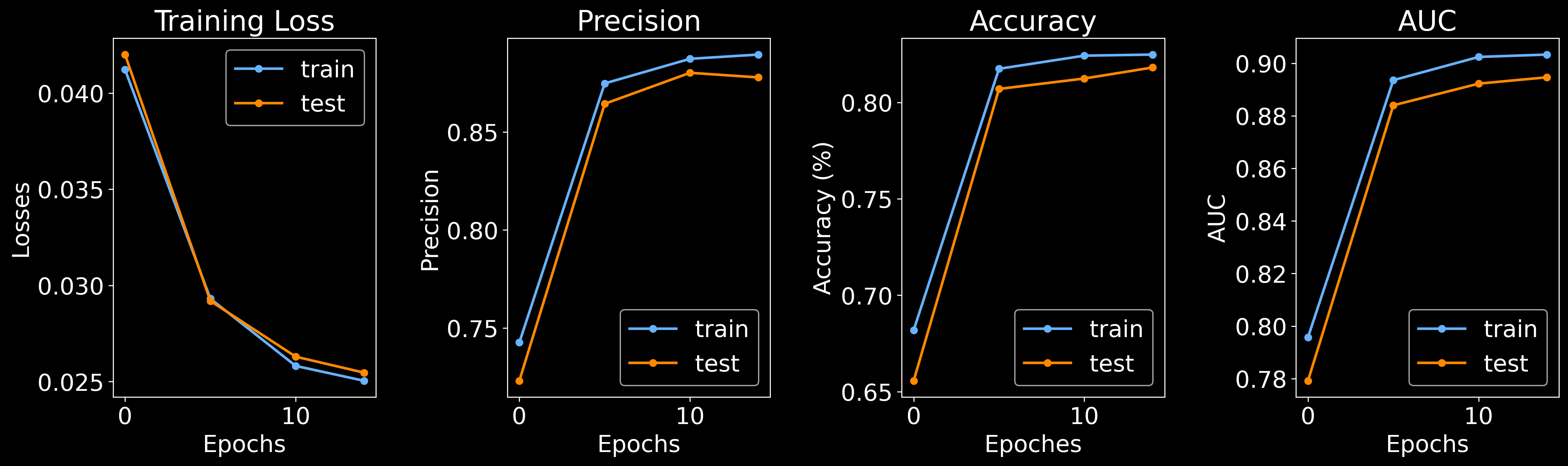
br.train.Training(
    bg,
    node_epoches = 50,
    edge_epoches = 15,
    edge_rbf_start = 0,
    edge_rbf_stop = 384,
    edge_rbf_n_kernels = 128,
)

Training node classifier:  98%|█████████████████████████████████████████████████████████████████████████████████████████████████  | 49/50 [00:49<00:00,  1.32it/s]

Training node classifier: 100%|███████████████████████████████████████████████████████████████████████████████████████████████████| 50/50 [00:53<00:00,  1.07s/it]
Training edge classifier:  93%|████████████████████████████████████████████████████████████████████████████████████████████▍      | 14/15 [00:12<00:00,  1.15it/s]

Training edge classifier: 100%|███████████████████████████████████████████████████████████████████████████████████████████████████| 15/15 [00:15<00:00,  1.05s/it]

Visualizing model

# randomly select a cell
random_cell = cells = random.sample(bg.segmented.index.values.tolist(), 2)[1]

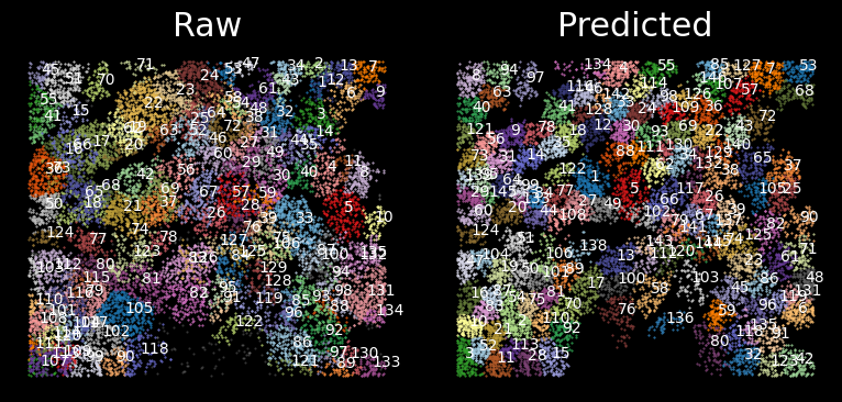
# plot node classification
df_window_raw, df_window_pred, predictions = br.pl.Plot_Classification(
    bg, 
    cell_name = random_cell,
    n_neighbors = 10, 
    zoomout_scale = 4,
)

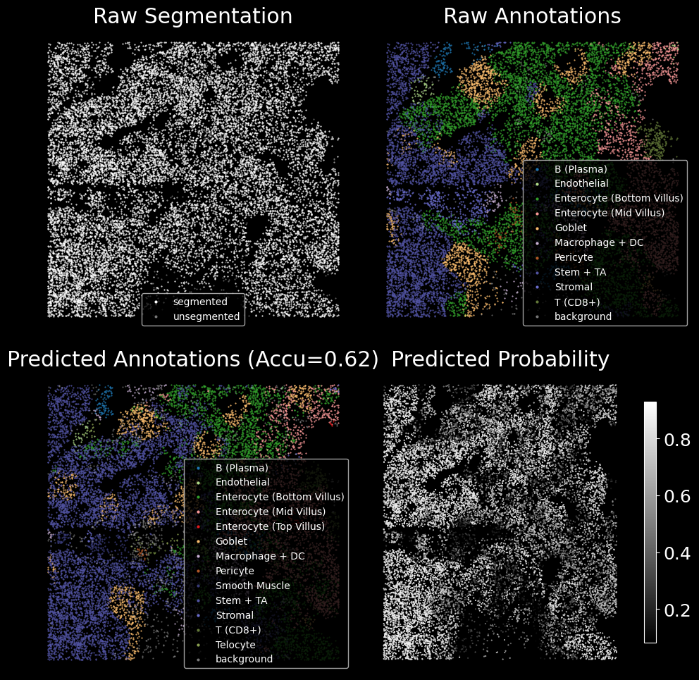
# plot cell segmentation
br.pl.Plot_Segmentation(
    bg, 
    cell_name = random_cell,
    df_window_raw = df_window_raw, 
    df_window_pred = df_window_pred,
    predictions = predictions,
    n_neighbors = 10, 
    zoomout_scale = 4,
    use_image = True,
    pos_thresh = 0.6,
    resolution = 0.5,
    num_edges_perSpot = 100,
    min_prob_nodeclf = 0.3,
    n_iters = 20,
)

After the model is trained, we can use the trained model to predict the cell types and segment all spots on the whole slice. After node classification and cell segmentation is completed, we generate single cell matrix in the end.

Node classification

Conduct node classification on the whole slice.

br.tl.node_classification(
    bg, bg.spots_all.copy(), 
    n_neighbors = 10, 
)
bg.spots_all.to_csv('spots_all.txt', sep = '\t')

Cell segmentation

br.tl.cell_segmentation(bg)

Get single cells

df_results, adata_ensembl, adata_segmented = br.tl.cell_annotation(bg)
df_results.to_csv('results.txt', sep = '\t')
adata_ensembl.write('results_cells_ensembled.h5ad')
adata_segmented.write('results_cells_segmented.h5ad')

print(f'Ensembled anndata: {adata_ensembl.shape}')
print(f'Segmented anndata: {adata_segmented.shape}')

... storing 'predicted_labels' as categorical

Ensembled anndata: (478, 241)
Segmented anndata: (951, 241)

Single cell data analysis

import scanpy as sc
sc.settings.set_figure_params(dpi=80)

# run standard analysis on the ensembled anndata
adata_ensembl = br.tl.cell_analyze(adata_ensembl)

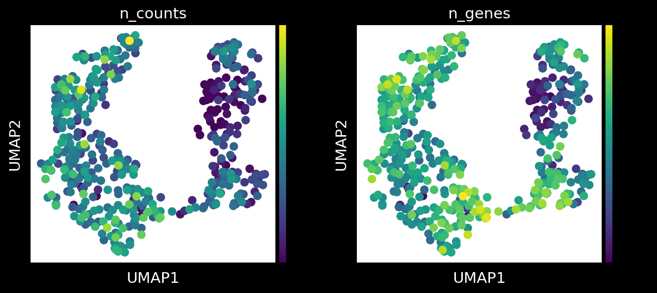
# first check the data quality of segmented cells
sc.pl.umap(adata_ensembl, color = ['n_counts','n_genes'])

2023-08-22 14:40:54.079668: I tensorflow/core/platform/cpu_feature_guard.cc:193] This TensorFlow binary is optimized with oneAPI Deep Neural Network Library (oneDNN) to use the following CPU instructions in performance-critical operations:  AVX2 AVX512F AVX512_VNNI FMA
To enable them in other operations, rebuild TensorFlow with the appropriate compiler flags.
2023-08-22 14:40:54.299465: I tensorflow/core/util/port.cc:104] oneDNN custom operations are on. You may see slightly different numerical results due to floating-point round-off errors from different computation orders. To turn them off, set the environment variable `TF_ENABLE_ONEDNN_OPTS=0`.

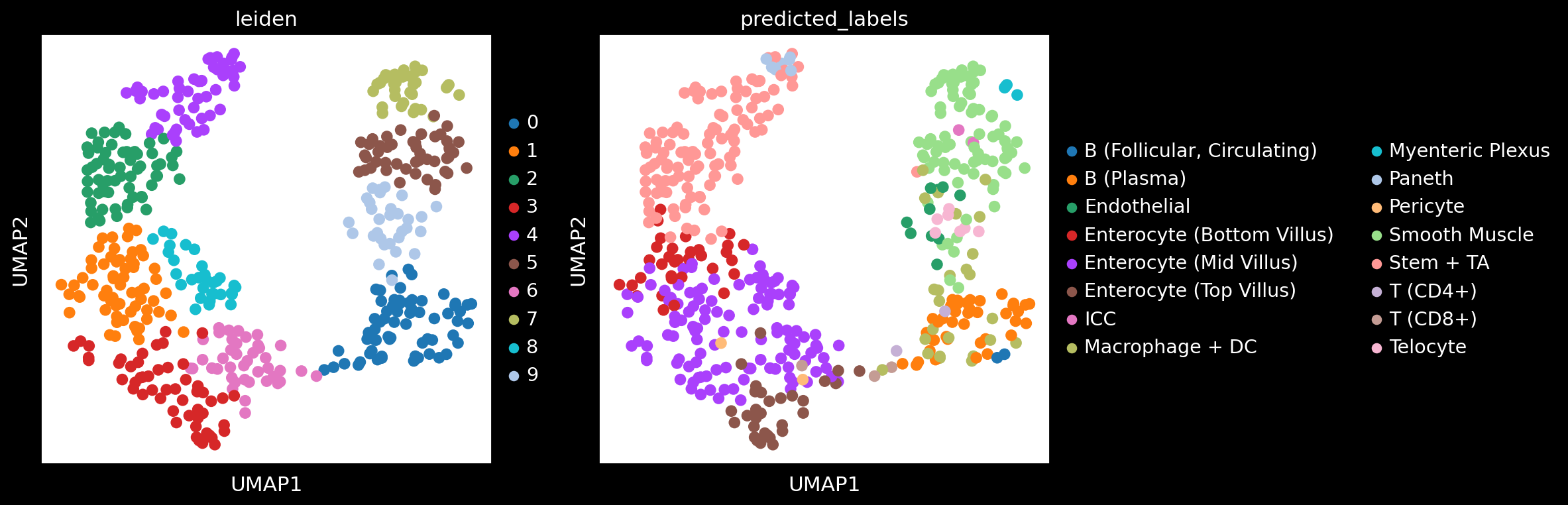
# plot leiden clustering and predicted labels from Bering
fig, axes = plt.subplots(1, 2, figsize = (15, 5))
axes[0] = sc.pl.umap(adata_ensembl, color = ['leiden'], ax = axes[0], show = False)
axes[1] = sc.pl.umap(adata_ensembl, color = ['predicted_labels'], ax = axes[1], show = False)

plt.subplots_adjust(wspace = 0.5)
plt.tight_layout()
plt.show()