%matplotlib inline

Analyze ISS hippocampal CA1 data

This tutorial shows how to apply Bering to ISS (pciSeq) CA1 data.

in-situ sequencing (ISS) hippocampal CA1 [Qian et al., 2020] data was derived from: https://doi.org/10.6084/m9.figshare.7150760.v1. We took one of the sample (sample 3-1 left CA-1) as an example in this tutorial.

Import packages & data

import random
import numpy as np
import pandas as pd
import matplotlib.pyplot as plt 

import Bering as br

# load data
df_spots_all = br.datasets.iss_ca1_qian()
df_spots_seg = df_spots_all[df_spots_all['labels'] != 'background'] # foreground nodes
df_spots_unseg = df_spots_all[df_spots_all['labels'] == 'background'] # background nodes
img = None
channels = None

df_spots_seg.head()

Downloading dataset `iss_ca1_qian` from `https://figshare.com/ndownloader/files/41409096` as `None.tsv`

	x	y	z	features	segmented	labels
0	209	441	0	Aldoc	67	Basket
2	215	450	0	Gad1	67	Basket
3	220	440	0	Pvalb	67	Basket
4	224	454	0	Slc24a2	67	Basket
5	229	438	0	Gad1	67	Basket

df_spots_unseg.head() # visualize unsegmented data

	x	y	z	features	segmented	labels
1	213	419	0	Pvalb	-1	background
16	270	383	0	3110035E14Rik	-1	background
17	282	436	0	Slc24a2	-1	background
18	287	342	0	3110035E14Rik	-1	background
19	290	436	0	Aldoc	-1	background

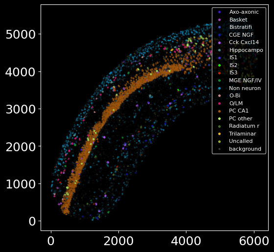
# visualize the spots
x, y = df_spots_seg['x'].values, df_spots_seg['y'].values
cell_types = df_spots_seg['labels'].values

fig, ax = plt.subplots(figsize = (6, 6))
for idx, cell_type in enumerate(np.unique(cell_types)):
    
    xc = x[np.where(cell_types == cell_type)[0]]
    yc = y[np.where(cell_types == cell_type)[0]]

    ax.scatter(xc, yc, s = 0.03, label = cell_type, color = np.random.rand(3,))

xb, yb = df_spots_unseg['x'].values, df_spots_unseg['y'].values
ax.scatter(xb, yb, color = '#DCDCDC', alpha = 0.2, s = 0.015, label = 'background')

h, l = ax.get_legend_handles_labels()
plt.legend(h, l, loc = 'upper right', fontsize = 8, markerscale = 15)

<matplotlib.legend.Legend at 0x2af736e73460>

Create Bering object

# image-dependent segmentation
bg = br.BrGraph(df_spots_seg, df_spots_unseg, img, channels)
bg

<Bering.objects.bering.Bering_Graph at 0x2af738f778b0>

bg.segmented.head() # summary of cells

	cx	cy	cz	dx	dy	dz	d	labels
segmented
0	236.0	442.0	0.0	41	31	0	41	Basket
1	295.0	467.0	0.0	38	29	0	38	Basket
2	312.5	351.0	0.0	41	28	0	41	PC CA1
3	320.0	394.0	0.0	24	25	0	25	PC CA1
4	330.0	296.0	0.0	32	18	0	32	PC CA1

Create training data

# Build graphs for GCN training purpose
br.graphs.BuildWindowGraphs(
    bg, 
    n_cells_perClass = 20, 
    window_width = 60.0, 
    window_height = 60.0, 
    n_neighbors = 10, 
)

br.graphs.CreateData(
    bg, 
    batch_size = 16, 
    training_ratio = 0.8, 
)

Training

br.train.Training(
    bg,
    edge_rbf_start = 0,
    edge_rbf_stop = 256,
    edge_rbf_n_kernels = 128,
)

Training node classifier:  98%|█████████████████████████████████████████████████████████████████████████████████████████████████  | 49/50 [00:26<00:00,  2.54it/s]

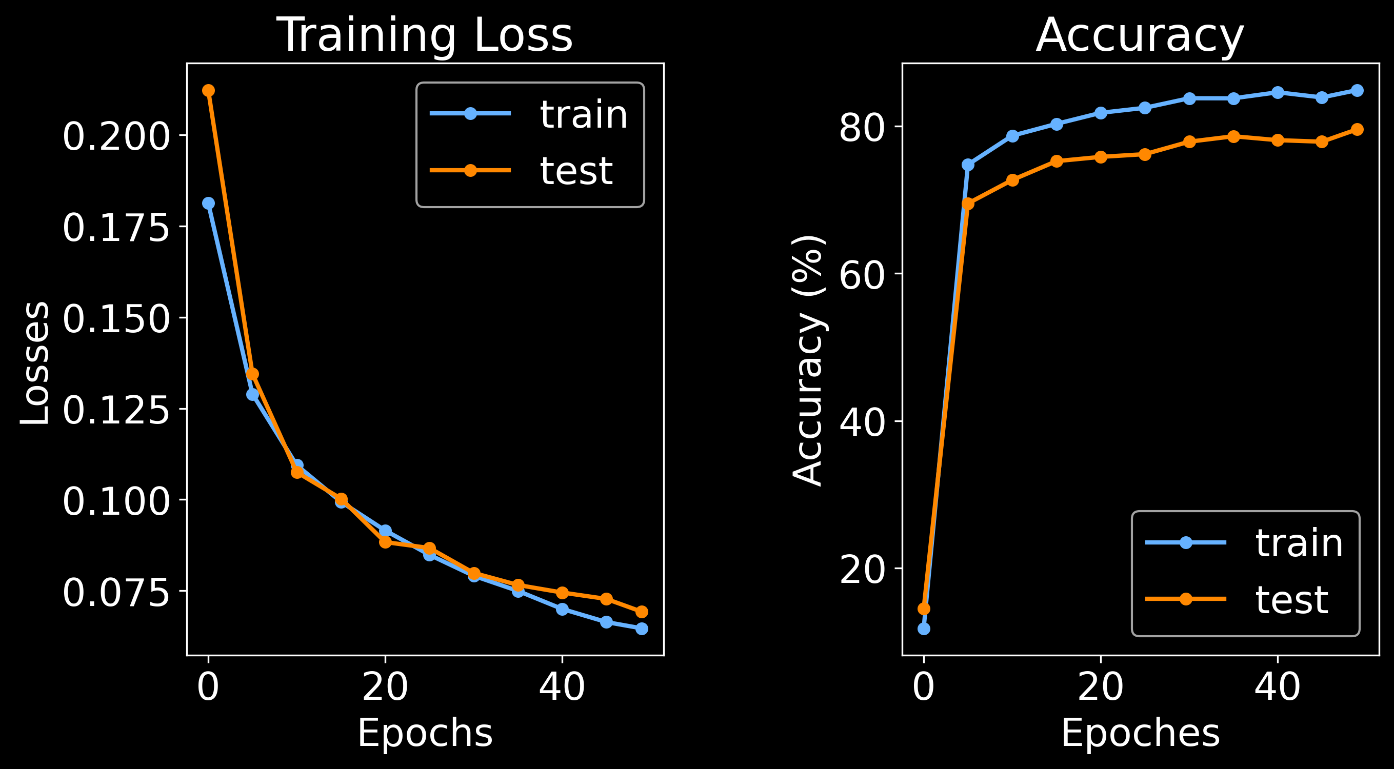
Training node classifier: 100%|███████████████████████████████████████████████████████████████████████████████████████████████████| 50/50 [00:29<00:00,  1.70it/s]
Training edge classifier:  98%|█████████████████████████████████████████████████████████████████████████████████████████████████  | 49/50 [00:28<00:00,  1.90it/s]

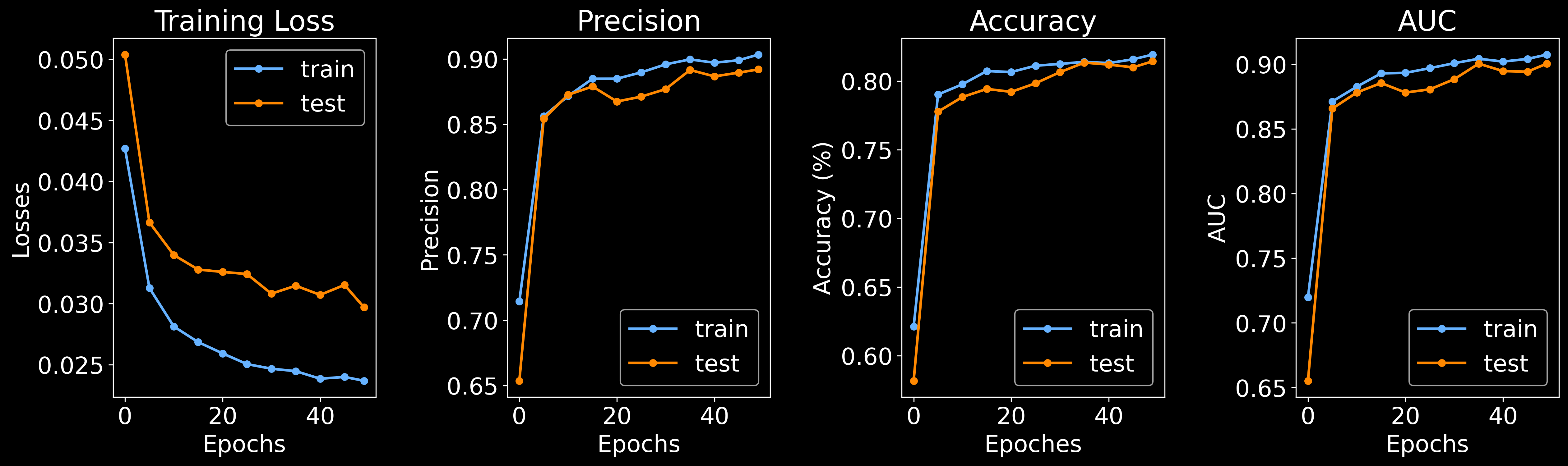
Training edge classifier: 100%|███████████████████████████████████████████████████████████████████████████████████████████████████| 50/50 [00:31<00:00,  1.61it/s]

# save the trained model
import pickle
with open('iss_ca1_qian.pkl', 'wb') as f:
    pickle.dump(bg, f)

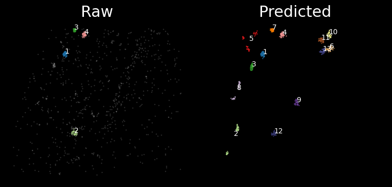
Visualizing model

# select middle cell
selected_cell = 362

# plot node classification
df_window_raw, df_window_pred, predictions = br.pl.Plot_Classification(
    bg, 
    cell_name = selected_cell,
    n_neighbors = 10, 
    zoomout_scale = 20,
)

# plot cell segmentation
br.pl.Plot_Segmentation(
    bg, 
    cell_name = selected_cell,
    df_window_raw = df_window_raw, 
    df_window_pred = df_window_pred,
    predictions = predictions,
    n_neighbors = 10, 
    zoomout_scale = 20,
    use_image = True,
    pos_thresh = 0.7,
    resolution = 0.3,
    num_edges_perSpot = 40,
    min_prob_nodeclf = 0.3,
    n_iters = 20,
)

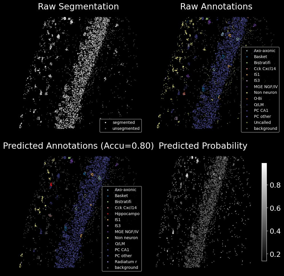
After the model is trained, we can use the trained model to predict the cell types and segment all spots on the whole slice. After node classification and cell segmentation is completed, we generate single cell matrix in the end.

Node classification

Conduct node classification on the whole slice.

br.tl.node_classification(
    bg, bg.spots_all.copy(), 
    n_neighbors = 10, 
)
bg.spots_all.to_csv('spots_all.txt', sep = '\t')

Cell segmentation

br.tl.cell_segmentation(
    bg,
    positive_edge_thresh = 0.6,
    leiden_resolution = 0.05,
    num_edges_perSpot = 100,
    graph_n_neighbors = 10,
    num_iters = 20,
)

Get single cells

df_results, adata_ensembl, adata_segmented = br.tl.cell_annotation(
    bg,
    min_dominant_nodes = 5, # set minimum number of nodes per cell as 8, so that we allow cells to be small in pciSeq
    min_dominant_ratio = 0.75,
)
df_results.to_csv('results.txt', sep = '\t')
adata_ensembl.write('results_cells_ensembled.h5ad')
adata_segmented.write('results_cells_segmented.h5ad')

print(f'Ensembled anndata: {adata_ensembl.shape}')
print(f'Segmented anndata: {adata_segmented.shape}')

... storing 'predicted_labels' as categorical

Ensembled anndata: (134, 80)
Segmented anndata: (1022, 84)

Single cell data analysis

import scanpy as sc
sc.settings.set_figure_params(dpi=80)

# run standard analysis on the ensembled anndata
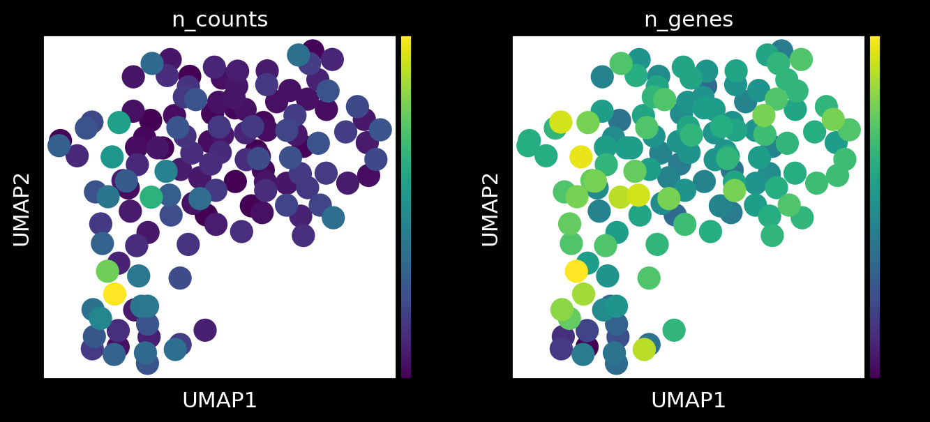
adata_ensembl = br.tl.cell_analyze(adata_ensembl, min_counts = 5)

# first check the data quality of segmented cells
sc.pl.umap(adata_ensembl, color = ['n_counts','n_genes'])

2023-08-22 17:43:26.681080: I tensorflow/core/platform/cpu_feature_guard.cc:193] This TensorFlow binary is optimized with oneAPI Deep Neural Network Library (oneDNN) to use the following CPU instructions in performance-critical operations:  AVX2 AVX512F AVX512_VNNI FMA
To enable them in other operations, rebuild TensorFlow with the appropriate compiler flags.
2023-08-22 17:43:27.644066: I tensorflow/core/util/port.cc:104] oneDNN custom operations are on. You may see slightly different numerical results due to floating-point round-off errors from different computation orders. To turn them off, set the environment variable `TF_ENABLE_ONEDNN_OPTS=0`.

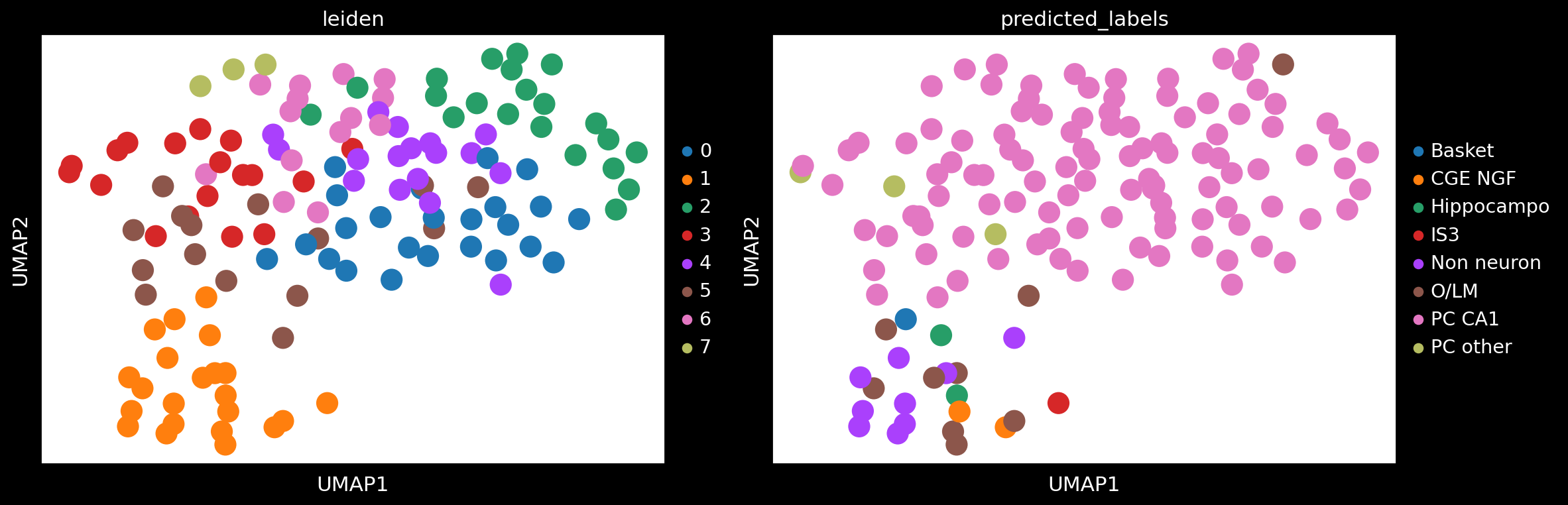
# plot leiden clustering and predicted labels from Bering
fig, axes = plt.subplots(1, 2, figsize = (15, 5))
axes[0] = sc.pl.umap(adata_ensembl, color = ['leiden'], ax = axes[0], show = False)
axes[1] = sc.pl.umap(adata_ensembl, color = ['predicted_labels'], ax = axes[1], show = False)

plt.subplots_adjust(wspace = 0.5)
plt.tight_layout()
plt.show()